In this post, we will explore an architectural approach known as Convolutional Neural Networks (CNNs), which is a crucial architecture extensively utilized in many deep learning applications. Therefore, we will meticulously examine the contents of the book, referred to as "Chris Bishop's 'Deep Learning - Foundations and concepts' ", to provide a comprehensive understanding of this important topic.
The necessity for convolutional networks arises from the requirement for a significantly large number of parameters in fully connected architectures when dealing with image data. Consider, for example, a color image with ${10^3} \times {10^3}$ pixels corresponding to red, green, and blue. If the networks. first hidden layer has 1000 hidden units, it would require $3 \times {10^3}$ weights. Moreover, learning inveriance and homogeneity through data necessitates an enormous dataset.
By designing architectures tailored to the structure of images, its possible to significantly reduce the dataset requirements and enhance generalization regarding the symmetry of image spaces. For instance, consider an image containing a face, which includes elements like eyes, and each eye contains structures like edges. At the lowest level of the hierarchical structure, nodes in the neural network can detect the presence of features such as edges using local information from small areas of the image, meansing it is only necessary to consider a small subset of the image pixels.
Using such structures, at higher levels of the hierarchy, it becomes possible to combine various features identified at previous levels to detect more complex structures. However, a critical point is that the details, including the types of features extracted at each level of the hierarchy, must be learned from the data.
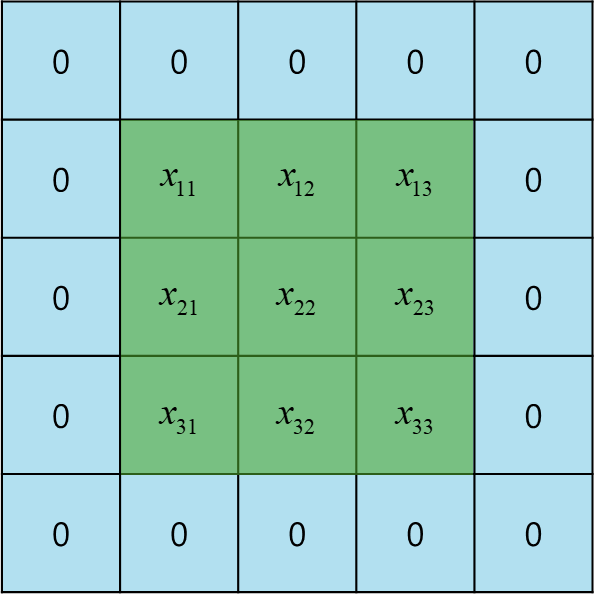
Consider a single unit in the first layer of a neural network dealing with an image that gas only one channel. This unit receives input solely from the pixel values within a small rectangular area or patch of the image. This patch is referred to as the receptive field of the unit, capturing the concept of locality. Moreover, the weights connected to this unit are trained to detect some useful low-level feature.
The output of this unit is typically represented in the form of a general function, consisting of a weighted linear combination of the inputs, which is then transformed using a nonlinear activation function.

Here, $\text{x}$ represents the vector of pixel values within the receptive field, and the activation function used as an example is the ReLU. Since there is one weight connected to each input pixel, these weights form a small two-dimensional grid, also referred to as a filter or kernel.

As seen in the picture, the convolutional map is smaller then the original image. If the image has dimensions of $J \times K$ pixels and is convolved with a kernal of dimensions $M \times M$, the resulting feature map will have dimensions of $(J - M + 1) \times (K - M + 1)$. Therefore, to prevent loss of information, a method of padding the original image with additioanl pixels around its perimeter is employed.
It the image is padded with $P$ pixels, the dimensions of the output map will be $(J + 2P - M + 1) \times (K + 2P - M + 1)$. When there's no padding, i.e., $P=0$, it's referred to as a valid convolution. To select a $P$ value that ensures the output array is the same size as the input, $P$ should be set to $(M - 1)/2$, which is termed as same convolution, because it results in the image and the feature map having the same dimensions. Typically, $M$ is chosen to be an odd number to apply symmetric padding to all sides of the image, ensuring a clear central pixel is defined in relation to the position of the filter.
The convolutional feature map has a similar size to the original image and will have the same size if identical padding is used. However, sometimes, for flexible design of the convolutional network architecture, it might be necessary to use feature maps that are larger than the original image. In such cases, strided convolution is used. Here, instead of moving across the image one pixel at a time, a larger step size, $S$(stride), is taken.
Using the same stride for both width and height allows the number of elements in the feature map to be calculated as follows.
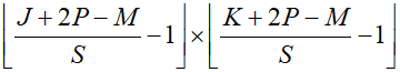
For large images and small filter sizes, the image map becomes approximately $1/S$ the size of the original image in terms of its dimensions.
'Deep Learning' 카테고리의 다른 글
| 71_Graph Convolutional Network (0) | 2024.02.09 |
|---|---|
| 70_Graph Neural Networks (0) | 2024.02.08 |
| 68_Residual Connection (0) | 2024.02.06 |
| 67_Automatic Differentiation (1) | 2024.02.05 |
| 66_Jacobian and Hessian Matrix (1) | 2024.02.04 |