As explained in the previous post, image processing can be performed using Convolutional Neural Networks (CNNs) through graphs. By treating pixels as nodes and edges as pairs of adjacent pixels in the image, an image can be viewed as a specific instance of graph-structured data.
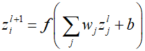
Here, $f$ represents a differentiable non-linear activation function, and because the same function is applied across various patches of the image, the weights ${w_j}$ and bias $b$ are shared among patches. However, the above equation is not equivariant to the permutation of the nodes' order in layer $l$, since the elements of the weight vector ${w_j}$ are not invariant to permutation. Therefore, initially considering the filter as a graph, we separate the contribution of node $i$ and assume that the other eight nodes are its neighbors, sharing a single weight parameter among neighbors.

Here, ${w_{self}}$ is the self-weight parameter for node $i$. Through the above formulation, it can be seen that the parameters ${w_{nei}}$, ${w_{self}}$, and $b$ are shared across all nodes, aggregating information from neighboring nodes. This setup ensures invariance to any permutation of the labels associated with the respective node, demonstrating that the model's predictions are consistent regardless of how the nodes are ordered.
Now, using a convolutional example, we aim to construct a deep neural network for graph-structured data. Through the formula mentioned, information is collected and combined from neighboring nodes, and then the node is updated as a function of the current node's embedding and the incoming messages. Thus, each processing layer can be seen as comprising two consecutive steps. The first step is the aggregation phase, where for each node $n$, messages are passed from neighboring nodes to form a new vector $z_{n}^l$ in a permutation-invariant way.
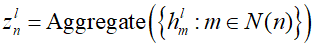
Through the equation, the node vector is aggregated from all neighbors of a specific node $n$ in the graph. The subsequent second step is the update phase, where the aggregated information from neighboring nodes is combined with the node's own local information to calculate the updated embedding vector for that node.

The method of applying convolution operations to graphs, known as graph convolution, is performed through the Fourier transform using the eigenvectors of the graph Laplacian, which is derived from the degree matrix minus the adjacency matrix of the graph. This can be represented by the following equation.

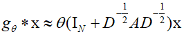
Here, $x$ represents the feature vector of each vertex, ${g_\theta}$ is the filter function represented as a diagonal matrix, and $U$ is the matrix whose columns are the eigenvectors of the graph Laplacian. However, the eigen decomposition of the graph Laplacian matrix is computationally complex and time-consuming. To simplify the computation, ${g_\theta}$ can be simplified to a first-order polynomial, and by scaling the graph Laplacian matrix to have its largest eigenvalue as 2, thereby scaling the Laplacian matrix between 0 and 1, the computation can be simplified.

Here, $D$ is the degree matrix of the graph, $A$ is the adjacency matrix, $L$ is the normalized graph Laplacian, and $\theta _0^`,\theta _1^`$ are the trainable graph convolution parameters, which can be modified as follows.
Applying the above formula repeatedly can lead to issues such as vanishing or exploding gradients, resulting in non-convergence. Therefore, through renormalization, the state embedding $H$ can be redefined as follows.

Where $W$ is the linear transformation matrix, which can be updaed through the following formula.

Here, $\sigma $ represents a nonlinear activation function, and $\tilde D$ is the diagonal matrix composed of the sum of each row of $\tilde A$, indicating how many neighbors each vertex has. The above formula, when expressed as a per-vertex update representation, can be articulated as follows.

Here, represents the set of vertex $i$ and its neighbors, where vertex $i$ calculates its new state using the information ($H_i^{k - 1}$) from all neighboring nodes connected to it.
'Deep Learning' 카테고리의 다른 글
| 73_Diffusion Model (0) | 2024.02.11 |
|---|---|
| 72_Generative Adversarial Networks (1) | 2024.02.10 |
| 70_Graph Neural Networks (0) | 2024.02.08 |
| 69_Convolutional Filter (0) | 2024.02.07 |
| 68_Residual Connection (0) | 2024.02.06 |