In the previous post, I described how to fine the derivatives of the weights through backpropagation of the network. In this post, I'll write about the process of calculating the Jacobian matrix, which is given as the derivative of the network's output with respect to the input through backpropagation, and the Hessian matrix, which is a second-order derivative.

Each derivative is calculated while keeping the other input values fixed, and the Jacobian matrix is useful in systems composed of several different modules. Assuming that we minimize the error function $E$ with respect to the paramter $w$, the derivative of the error function is as follows.

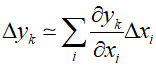
The Jacobian matrix measures the local sensitivity of the outputs to changes in each input variable. Therefore, a known error $\Delta {x_i}$ associated with an input can be propagated through the trained network to estimate the contribution to the error in the output $\Delta {y_k}$, as represented by the following relationship.
Typically, the above equation is only useful for mall variations in input values, and the Jacobian itself must be re-evaluated for each new input vector.
The Jacobian matrix can be evaluated using a backpropagation procedure similar to that used for evaluatin the derivatives of various functions with respect to the weights. The ${J_{ki}}$ element can be written in the following form.

The sum in the above equation is taken over all units $j$ to which the input unit $i$ sends connections. Also, the recursive backpropagation formula for the derivative $\partial {y_k}/\partial {a_j}$ is as follows.

In the above equation, the sum is taken over all units $l$ to which unit $j$ sends connections. Also, the formula described in the previous post(65_Backpropagation)is used. This backpropagation starts at the output units, and the necessary derivatives can be found directly from the functional form of the output unit activation function. In the case of linear output units, it is as follows.

Where ${\delta _{kl}}$ is an element of the identity matrix. If each output unit has an individual logistic sigmoid activation function, it would be as follows.

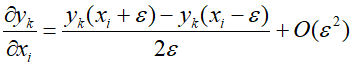
To evaluate the Jacobian matrix at a point in the input space corresponding to an input vector, it is typically necessary to forward propagate to obtain the states of all hidden and output units in the network. Then, the previously described formulas are used. The implementation of such an algorithm can also be calculated using the following numerical differentiation.
Similarly, backpropagation can also be used to evaluate the second-order derivatives of the error, as follows.

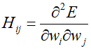
When all weight and bias parameters are combined into the elements ${w_i}$ of a single vector $w$, the second derivatives form theelements ${H_{ij}}$ of the Hessian matrix $H$.
The Hessian matrix is used in a variety of places including several nonlinear optimization algorithms for neural network training, Bayesian neural network processing, and optimization of large language models. The efficiency of evaluating the Hessian is an important consideration. If there are $W$ parameters in the network, the Hessian matrix has dimensions $W \times W$, which means the computational cost required to evaluate it at each point in the dataset increases by $O({W^2})$
Additionally, since neural networks can contain millions or even billions of parameters, evaluating the full Hessian matrix for many models is impractical. Therefore, approximations for the full Hessian are sought to reduce computational costs.
Considering regression using the sum-of-squares error function, it can be described as follows.

For simplicity of notation, considering a single output, the Hessian matrix can be written as follows.
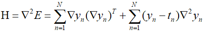
Where $\nabla $ is represents the gradient with respect to $w$. If the output ${y_n}$ is very colse to the target velue ${t_n}$, the last term can be neglected. In such a case, we obtain the Levenberg-Marquardt approximation, which is also known as the "outer product approximation" because the Hessian matrix is composed from a sum of outer products of vectors, as follows.
Evaluating the outer product approximation of the Hessian is straightforward as it involves only the first-order derivatives of the error function and can be performed in $O(W)$ steps using standard backpropagation. The elements of the matrix can be found through multiplication. The approximation for the cross-entropy error function of a network with logistic sigmoid output unit activation functions is as follows.

'Deep Learning' 카테고리의 다른 글
| 68_Residual Connection (0) | 2024.02.06 |
|---|---|
| 67_Automatic Differentiation (1) | 2024.02.05 |
| 65_Backpropagation (0) | 2024.02.03 |
| 64_Normalization (0) | 2024.02.02 |
| 63_Learning Rate Schedule (0) | 2024.02.01 |