It has been emphasized that using gradient information is crucial for efficiently training neural networks. While there are many methods to evaluate the gradient of a neural network's error function, one method worth exploring is "automatic differentiation" or "autodiff".
Unlike symbolic differentiation, the goal of automatic differentiation is not to find the mathematical expression of the derivative, but to enable the computer to automatically generate gradient calculations with only the code for the forward propagation equations. This approach is as accurate as symbolic differentiation but more efficient, as it utilizes intermediate variables to avoid redundant calculations.
The core idea of automatic differentiation is to take the code that computes a function and supplement it with additional variables that accumulate values during code execution to obtain the corresponding derivatives. There are primarily two forms: forward mode and reverse mode. Let's first explain the forward mode.
In forward mode automatic differentiation, each intermediate variable ${z_i}$ participating in the evaluation of the function is considered as a 'primal' variable, and an additional variable ${\dot z_i}$, representing the derivative value of that variable, is considered as a 'tangent' variable. Instead of simply performing forward propagation to calculate $\{ {z_i}\} $, tuples $({z_i},{\dot z_i})$ are propagated so that both the variable and its derivative are evaluated in parallel. This derivative can then be used in conjunction with the chain rule to automatically generate code for calculating gradients.
For example, consider a function with two input variables as follows.

When implementing automatic differntiation, the code is structured in the squence of operations that can be represented as an evaluation trace of basic operations, and the primal variables are defined as follows.

To calculate the derivative $\partial f/\partial {x_1}$, define the tangent variable as ${\dot v_i} = \partial {v_i}/\partial {x_1}$. Then, using the chain rule of calculus, the calculation can be expressed as follows.

Where ${\text{pa}}(i)$ represents the set of parent node of node $i$. Using the primal variables in the above equation, the quation for the tangent variables can be obtained as follows.

Therefore, to summarize the automatic differentiation for the above formula, first write the code that implements the evaluation of the primal variables, and then compute the tangent cariables. To evaluate the derivative $\partial{f}/\partial {x_1}$, input specific values for ${x_1}$ and ${x_2}$, and numerically calculate the tuple $({v_i},{\dot v_i})$ based on the primal and tangent equations. This process yields the required derivative, ${\dot v_5}$.
Considering an example with two outputs, ${f_1}({x_1},{x_2})$ and ${f_2}({x_1},{x_2})$, where ${f_1}({x_1},{x_2})$ is as previously defined, and ${f_2}({x_1},{x_2})$ is as follows.

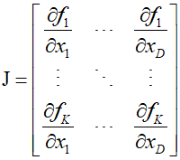
This requies only a slight extension of the primal and tangent variable evaluation equations, allowing both $\partial{f_1}/\partial {x_1}$ and $\partial{f_2}/\partial {x_1}$ to be evaluated in a single forward pass. The evaluation of the derivative with respect to ${x_2}$ requires a separate forward pass. Generally, for a function with $D$ inputs and $K$ outputs, forward mode automatic differentiation produces a single column of the Jacobian matrix of size $K \times D$.
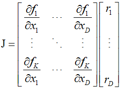
To compute column $j$ of the Jacobian, it is necessary to set ${\dot x_j} = 1$ and ${\dot x_i} = 0$ for $i \ne j$ to initialize the forward propagation of the tangent equations. This can be written in vector form as $\dot x = {{\text{e}}_i}$. to compute the full Jacobian matrix, $D$ forward passes are required, and the multiplication of the Jacobian with a vector ${\text{r}} = {({r_1}, \cdots ,{r_D})^T}$ can be computed as follows.
Reverse mode automatic differentiation is a generalization of the error backpropagation procedure and, like the forward mode, adds additional variables to each intermediate variable ${v_i}$. These additional variables are called 'adjoint variables' and are denoted as ${{\bar v}_i}$. In the situation with a single output function $f$, the adjoint variables are defined as follows, and can be calculated sequentially in reverse order from the output using the chain rule of calculus.
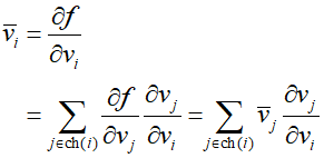
Where ${\text{ch}}(i)$ represents the child nodes of node $i$. The evaluation equations for the above formulas are as follows, representing the reverse flow of information through the graph.

Reverse mode starts from the output and proceeds backwards to the input. In the case of multiple inputs, only a single reverse pass is needed to evaluate the derivatives, but for multiple outputs, a separate reverse pass must be executed for each output variable. Generally, it is easier to implement forward mode than reverse mode because, during the reverse pass, all intermediate primal variables needed to compute the adjoint variables must be stored. In contrast, in forward mode, the primal and tangent variables are calculated together during forward propagation and can be discarded after use. However, both modes typically cost only about 2 to 3 times more than the computation cost of a single function evaluation.
ref : Chris Bishop's "Deep Learning - Foundations and Concepts"
'Deep Learning' 카테고리의 다른 글
| 69_Convolutional Filter (0) | 2024.02.07 |
|---|---|
| 68_Residual Connection (0) | 2024.02.06 |
| 66_Jacobian and Hessian Matrix (1) | 2024.02.04 |
| 65_Backpropagation (0) | 2024.02.03 |
| 64_Normalization (0) | 2024.02.02 |