In deep neual networks, increasing the number of layers in the network can improve generalization performance. Additionally, batch normalization can mitigate the problems of vanishing and exploding gradients. However, even with batch normalization, training a network with many layers is challenging.
The representational power of a neural network increase exponentially with its depth. However, the discontinuities in the error function's gradient also increase correspondingly. The differentiation of the network is expressed in terms of the input function's variables and determines the gradient of the error function surface by the chain rule of calculus. Therefore, in the case of deep neural networks. very small changes in the weight parameters of the initial layers of the network can cause significant changes in the gradient.
Therefore, iterative gradient-based optimization algorithms requires the assumption that gradients change smoothly across the paramter space, and such fragmented gradients make training highly inefficient in very deep neural networks.
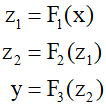
Here, residual connections can greatly benefit neural network architecture. Residual connections are a specific form of skip-layer connections. To illustrate, consider a neural network composed of three as follows.

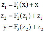
Here the function $\text{F}$ can simply be a complex function that includes a sequence of operations such as linear transformations followed by various linear, activation, and normalization layers. Residual connections are made by simply adding the input back to the output of each function.


Combinations of functions and residual connections, such as ${{\text{F}}_1}({\text{x}}) + {\text{x}}$, are known as residual blocks. Networks known as Residual Networks or ResNets consist of multiple layers of these blocks in sequence. Residual blocks can easily create an identity transformation when the parameters within the nonlinear functions are sufficiently small, making the function's output nearly zero. The trem 'residual' implies that each block learns the residual between the identity map and the desired output. This can be reformulated as follows.

The above equation represents a residual transformation. Networks wit residual connections are much less sensitive to input values compared to conventional deep networks. Typically, residual networks incorporate batch normalization layers, and using these two techniques together can significantly reduce the problems of gradients vanishing and exploding. Combining the above equations to obtain a single overarching equation for the entire network can be represented as follows.

Here, by substituting the intermediate variables ${{\text{z}}_{\text{1}}}$ and ${{\text{z}}_{\text{2}}}$, an expression for the network output with respect to the input ${\text{x}}$ can be obtained.

In this extended form of the residual netwrok, the entire function is composed of multiple networks operating in parallel. Since the input and all intermediate variables must have the same dimension, skip connections as defined by the above equations can be added. The dimension at any point in the network can be altered through the use of a non-square matrix ${\text{W}}$ of trainable parameters.

Here, the function ${{\text{F}}_l}$ is a learnable nonlinear function, and it refers to a standard neural network that alternates between layers composed of learnable linear transformations and fixed nonlinear activation functions.
Refference
Balduzzi, David, et al. "The shattered gradients problem: If resnets are the answer, then what is the question?." International Conference on Machine Learning.PMLR, 2017.
He, Kaiming, et al. "Deep residual learning for image recognition." Proceedings of the IEEE conference on computer vision and pattern recognition. 2016.
'Deep Learning' 카테고리의 다른 글
| 70_Graph Neural Networks (0) | 2024.02.08 |
|---|---|
| 69_Convolutional Filter (0) | 2024.02.07 |
| 67_Automatic Differentiation (1) | 2024.02.05 |
| 66_Jacobian and Hessian Matrix (1) | 2024.02.04 |
| 65_Backpropagation (0) | 2024.02.03 |