In this post, the focus is on efficiently finding the gradient of the error function $E(w)$ of a feedforward neural network. This can be achieved by sending information backward through the network, a process also known as error backpropagation. The term 'backpropagation' is used to clearly describe the procedure for numerically evaluating derivatives, such as the gradient of the error function with respect to the weights and biases of the network.
Typically, a feedforward network involves each unit calculating a weighted sum of its inputs, which can be represented by the following equation.

Where ${z_i}$ is the activation of the input unit that sends connections to another unit, and ${w_{ji}}$ is the weight associated with that connection. The above equation represents the pre-activation, which is transformed by the nonlinear activation function $h$ to form the activation ${z_j}$, as follows.

For each data point in the training set, providing the corresponding input vector to the network and calculating the activations of all the hidden and output units of the network through the continuous application of the above equations is considered as information being transmitted through the network. This process is referred to as forward propagation.
The output of various units changes depending on a specific input data point $n$. Initially, ${E_n}$ depends on the weighted sum of inputs ${a_j}$ for unit $j$, which in turn depends on the weight ${w_ji}$. Thus, applying the chain rule for partial derivatives with respect to ${w_{ji}}$, we get the following.
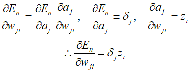
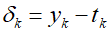
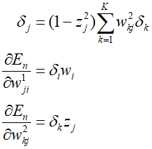
From the above equation, we can see that the required derivative is obtained by multiplying the value of $\delta $ for the unit at the output end of the weight with the value of $z$ for the unit at the input end of the weight. Therefore, to evaluate the derivative, we neeed to calculate the value of ${\delta _j}$ for each hidden and output unit of the network and apply the formula. For the output units, it can be represented as follows.
To evaluate $\delta $ for hidden units, we use the chain rule for partial derivatives again.

From the above equation, we can see that a change in ${a_j}$ only causes a change in the error function through the variable ${a_k}$. Therefore, summarizing the above formulas, we can obtain the backpropagation formula as follows.
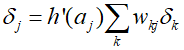
This means that the value of $\delta $ for a specific hidden unit can be obtained by propagating backwards from the units above it in the network. Assuming that the $\delta $ values for the output units are known, the recursive application of the above formula allows for the calculation of $\delta $ values for all hidden units in the feedforward network.
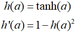
To illustrate the application of the algorithm thus far, let's consider a network with two layers and the sum-of-squares error as an example. The output units have a linear activation function, so ${y_k}={a_k}$, and sigmoid activation function of the hidden units is as follows.
Considering the sum-of-squares error function, the error for data point $n$ is as follows.
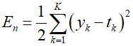
Where ${y_k}$ is the activation value of output unit $k$, and ${t_k}$ is the target value for the corresponding input vector ${x_n}$.. For each data point, forward propagation is performed using the data points of the training set.

Where $D$ is the dimension of the input vector, and $M$ is the total number of hidden units. Also, ${x_0}={z_0}=1$. The value of $\delta$ for each output unit is as follows.

Subsequently, through backpropagation, the $\delta$ values for the hidden units are calculated, and the derivatives for the weights of the first and second layers can also be determined.
'Deep Learning' 카테고리의 다른 글
| 67_Automatic Differentiation (1) | 2024.02.05 |
|---|---|
| 66_Jacobian and Hessian Matrix (1) | 2024.02.04 |
| 64_Normalization (0) | 2024.02.02 |
| 63_Learning Rate Schedule (0) | 2024.02.01 |
| 62_Gradient Information (0) | 2024.01.31 |