Based on what we studied in the previous post, I'll solve an example problem.

In the figure above, we calculate the temperature distribution along the insulated external boundary.
The temperature at the left end is fixed at ${40^ \circ }{\text{C}}$, and the free-stream temperature is ${-10^\circ}{\text{C}}$. The value of $h$ is ${\text{55W(}}{{\text{m}}^{\text{2}}}{{\text{ - }}^{\text{o}}}{\text{C)}}$, and the value of ${K_{xx}}$ is ${\text{35W(}}{{\text{m}}^{\text{2}}}{{\text{ - }}^{\text{o}}}{\text{C)}}$. Here, $h$ represents forced air convection, and ${K_{xx}}$ is the conductivity for carbon steel.
The rod will be divided into four elements each of $0.25m$ in length for the calculation. The left end of the rod has a fixed temperature, and the top and bottom are insulated, so convective heat loss only occurs at the right end.
Calculating the stiffness matrix for each element, it is as follows.
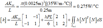
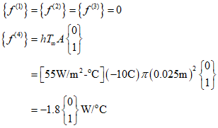
By arranging the above equation, we can obtain the expression for the first element, which is zero due to the absence of a convection term. The second and third elements are also the same.

However, the fourth element has a convection term since there is heat loss at the right end.

In this example, the element force matrix has $Q=0$(no heat source), ${q^*}=0$(no heat flux), and since there is convection only at the right end, it can be calculated as follows.
By assembling the element stiffness matrix and the element force matrix, the following system of equations can be obtained.
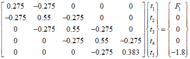
Where ${F_1}$ is the heat flow rate at the first node, and since we know that ${t_1} = {40^{\text{o}}}{\text{C}}$ at the first node, such non-homogeneous boundary condition problems can be handled in the same way as stress analysis problems.
Therefore, it can be modified as follows.
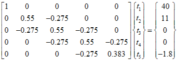
Therefore, since there are five equations and five unknowns, the solution can be calculated as follows.

'Finite Element Method' 카테고리의 다른 글
| 47_2-D Heat Transfer Finite Element Formulation (0) | 2024.01.16 |
|---|---|
| 46_1-D Heat Transfer Example(2) (0) | 2024.01.15 |
| 44_1-D Heat Transfer Finite Element Formulation(2) (1) | 2024.01.13 |
| 43_1-D Heat Transfer Finite Element Formulation (0) | 2024.01.12 |
| 42_One-Dimensional Heat Conduction (1) | 2024.01.11 |