I plan to study diffusion models, which are widely used method for constructing generative models that involve findinf a distribution $p({\text{z)}}$ for the latent variables ${\text{z}}$ and using deep neural networks to transform ${\text{z}}$ into the data space ${\text{x}}$.
Diffusion models work by gradually adding noise to trained images, transforming them into samples of Gaussian distribution, and a deep neural network is trained to reverse this process. After training, the network can take Gaussian samples as input to generate new images.
Diffusion models are fixed generative distributions defined by a noise process and provide results of similar or better quality than Generative Adversarial Networks, which were covered in a previous post. However, generating new samples can be computationally expensive because it requires multiple forward passes through the decoder network.
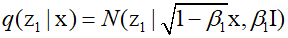
First, take an image from the training set and mix Gaussian noise into each pixel to create a noise-added image ${{\text{z}}_1}$.

Here, ${{{\epsilon}}_1}$ is noise following a Gaussian distribution, and ${{\beta _1}}<1$ is the variance of the noise distribution. The above equation can be written in the following form.
Subsequently, by repeating this process with additional independent Gaussian noise steps, images with more noise are obtained. The latent variables are denotes as ${\text{z}}$, and the observed variables are denoted as ${\text{x}}$. Each successive image is given as follows.
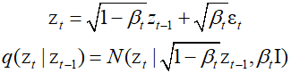
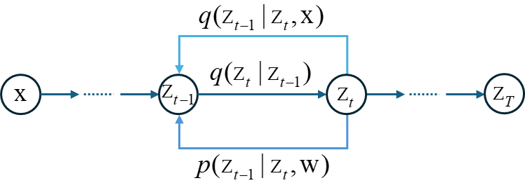
The sequence of conditional distributions forms a Marcov chain and can be represented as a graphical model. The values of the variance parameters are set manually, and typically, the variance values increase with $t$.
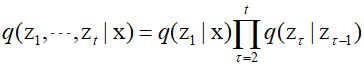
For the observed data vector ${\text{x}}$, the joint distribution of the latent variables is as follows.
By marginalizing over the intermediate variables ${\text{z}}$, the diffusion kernel can be obtained.

Each intermediate distribution has a simple colsed-form Gaussian expression, enabling stochastic gradient descent using any intermediate term of the Markov chain without running the entire chain.

${{\varepsilon }}$ represents the total noise added to the original image, not the incremental noise added at each step of the Markov chain. After many steps, the image becomes indistinguishable from Gaussian noise, and in the limit as $T \to \infty $, it is as follows.

Therefore, the coefficients $\sqrt {1 - {\beta _t}} $ and $\sqrt {{\beta _t}} $ ensure that after coverging to a distribution with a mean of 0 and unit coveriance, additional update do not alter it through the Markov chain.
To reverse the noise process, one must consider the inverse of the conditional distribution. This can be expressed using Bayes' theorem as follows.

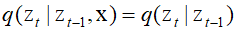
Here, $q({{\text{z}}_{t - 1}}|{\text{x}})$ is given as a conditional Gaussian distribution. However, this distribution is difficult to compute because it requires integration over an unknown data density. Instead, one considers the reverse-direction distribution conditioned on the data vector ${\text{x}}$. This distribution is defined as $q({{\text{z}}_{t - 1}}|{{\text{z}}_t}{\text{,x}})$ and simplifies the problem if the starting image is known given a noisy image. Using Bayes' theorem, this conditional distribution can be computed.

Using the Markov property, it can be written as follows.
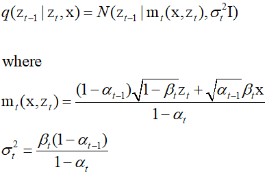
Through the above equations, the right side, which takes the form of a Gaussian distribution, can be analyzed using the method of completing the square to finethe mean and coveriance.
'Deep Learning' 카테고리의 다른 글
| 97_Simple ANN Example Using PyTorch (0) | 2024.03.06 |
|---|---|
| 74_Diffusion Model(2) (0) | 2024.02.12 |
| 72_Generative Adversarial Networks (1) | 2024.02.10 |
| 71_Graph Convolutional Network (0) | 2024.02.09 |
| 70_Graph Neural Networks (0) | 2024.02.08 |