Similar to regression and classification models, model parameters are defined by optimizing an error function. optimization can be efficiently performed using gradient information, making it essential for the function to be diffferentiable. Here, the derivative is calculated using backpropagation, and the details of backpropagation will be covered later.
Finding the optimal values for the weights and biases of a neural network is reffered to as training the model. For convenience, there parameters are often grouped into a single vector, and optimization is performed using an error function. Initially, by adding a small region $\delta {\text{w}}$ in the weight space ${\text{w}}$ to represent ${\text{w}}+\delta {\text{w}}$, the change in the error function can be expressed as follows.

Where $E$ is the error function, and the vector $\nabla E$ points in the direction of the greatest increase of the error function. If the error function is differentiable, the smallest value occure at a point in the space where the gradient vanishes.

The goal of learning is to find the vector ${\text{w}}$ that makes $E({\text{w}})$ as small as possible. The smallest value of the error function in the entire space of ${\text{w}}$ is referred to as the global minimum, while smaller minimum values in specific regions of ${\text{w}}$ are called local minimum. It is not always possible to fine the global minimum, and often the process may settle in a local minimum.
The Taylor expansion of the error function around a point ${\hat{\text {w}}}$ in the weight space is as follows.
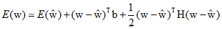
This approximation includes terms up to the second orer, where ${\text{b}}$ is defined as the gradient of $E$ evaluated at ${\hat{\text {w}}}$.

Here, ${\text{H}}$ is the Hessian, represented by second-order derivatives. If there are a total of ${\text{W}}$ weights and biases in the network, both ${\text{w}}$ and ${\text{b}}$ are vectors of length ${\text{W}}$, and ${\text{H}}$ is a matrix of size ${\text{W \times W}}$. According to the Taylor expansion, the gradient can be approximated as follows.

For a quadratic approximation around the point ${{\text{w}}^*}$, which is the minimum of the error function, since $\nabla E = 0$, it can be summarized as follows.

Here, the eigenvalue equation for the ${\text{H}}$ matrix is as follows.

Additionally, the eigenvectors ${{\text{u}}_i}$ form an otrhonormal set.

$({\text{w}} - {{\text{w}}^*})$ can be expanded as a linear combination of eigenvectors.

Therefore, it is similar to a coordinate transformation that moves the origin to the point ${{\text{w}}^*}$ and aligns the axes with the eigenvectors. Summarizing the above equations, the error function can be written as follows.
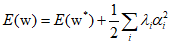
Where, if the eigenvalue $\lambda $ is positive, the error function increases, and if $\lambda $ is negative, it decreases. Furthermore, if all eigenvalues are positive, ${{\text{w}}^*}$ corresponds to a local minimum of the error function, and if all eigenvalues are negarive, it corresponds to a local maximum.
'Deep Learning' 카테고리의 다른 글
| 63_Learning Rate Schedule (0) | 2024.02.01 |
|---|---|
| 62_Gradient Information (0) | 2024.01.31 |
| 60_Multilayer Networks and Activation Function (0) | 2024.01.29 |
| 59_Generative Classifiers(2) (1) | 2024.01.28 |
| 58_Generative Classifiers (0) | 2024.01.27 |