While using higher-order shape functions has the advantage of more accurately approximating irregularly shaped curve boundaries, they are generally not used as frequently due to the increased computation time, with lower-order shape functions being the preferred choice.
In this post, the method for calculating higher-order shape functions will be explained.

As shown in the figure above, the aim is to determine the shape functions and the $B$ matrix for a linear bar isoparametric element with three nodes.
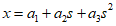
Using the natural coordinates $s$ values for the given three nodes, the shape function for the x-coordinate can be represented as follows.
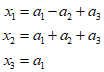
Additionally, the ${a_i}$ values using the node coordinates are as follows.
To summarize, it is as follows.

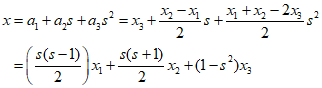
Substituting the summarized equation into the initial equation to express it in therms of $x$, it results as follows.
Sicne $x$ can be expressed through the relationship of the shape function matrix and the axial coordinates, it can be represented as follows.
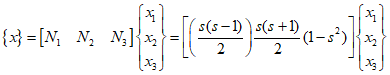
Therefore the shape functions are,

Now start with the basic definition of axial strain and calculate the $B$ matrix.
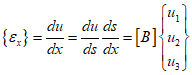
The isoparametric formulation can be represented as follows, as the displacement function has the same form as the axial coordinate function.
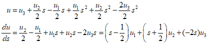
From the previous post, we know that $\frac{{dx}}{{ds}} = \frac{L}{2}$, and using this relationship, it can be summarized as follows.
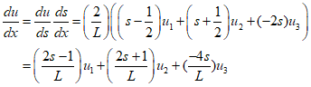
In matrix form,

Expressing the above equation for axial strain, it becomes,

'Finite Element Method' 카테고리의 다른 글
| 40_3-Dimensional Stress and Strain (0) | 2024.01.09 |
|---|---|
| 39_High Order Example (0) | 2024.01.08 |
| 37_Element Stress (1) | 2024.01.06 |
| 36_Gaussian Quadrature Example (0) | 2024.01.05 |
| 35_Gaussian Quadrature (2) | 2024.01.04 |