In engineering problems, nonlinear models oftern fit data better than linear models. These models can be defined as having nonlinear dependencies on their parameters.

For instance, such an equation typically cannot be transformed into the following form.

Like linear least squares, nonlinear regression also determines parameter values that minimize the sum of the squares of the residuals. However, in the nonlinear case, this usually requires iterative methods to solve.
One such algorithm is the Gauss-Newton method, which is used to minimize the sum of the squares of the residuals between the data and a nonlinear equation. The core concept of this method involves using the Taylor series expansion to represent the original nonlinear equation in an approximate linear form. Subsequently, the least squares theory is applied to minimize the residuals and obtain new estimates for the parameters.
To explain this, the relationship between the nonlinear equation and the data can generally be expressed as follows.
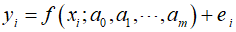
Where ${y_i}$ represents the measured values of the dependent variable, $f({x_i};{a_m})$ is a nonlinear function of the independent variable ${x_i}$ and parameters ${a_0},{a_1}, \cdots {a_m}$ and ${e_i}$ is the random error. For simplicity, the model can be abbreviated by omitting parameters, expressed in a condensed form.

In a nonlinear model, the function is expanded around the parameter values using a Taylor series, and terms beyond the first derivative are typically omitted.

Here, $j$ represents the initial estimate and $j+1$ is the prediction. Therefore, by linearizing the original model with respect to the parameters, it can be expressed as follows.

Alternatively, it can be represented in matrix form as follows.

Here, ${z_j}$ is the matrix of partial derivatives of the function calculated at the initial estimate $j$.

Where $n$ represent the number of data points, and $\partial {f_i}/\partial {a_k}$ is the partial derivative of the function with respect to the $k$th parameter at the $i$th data point. The vector $D$ denotes the difference between the measured values and the function values.

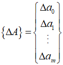
And $A$ represents the change in parameter values.
Applying linear least squares theory, the normal equations can be derived as follows.

Therefore, solve for $\Delta A$ from the above equation to calculate the improved values of the parameters.

Repeat this process until the solution converges, falling below an acceptable stopping criterion.

'Numerical Methods' 카테고리의 다른 글
| 149_Quadratic Interpolation (0) | 2024.04.27 |
|---|---|
| 148_Linear Interpolation (0) | 2024.04.26 |
| 146_Polynomial Regression (0) | 2024.04.24 |
| 145_Newton's Method (0) | 2024.04.23 |
| 144_Parabolic Interpolation (0) | 2024.04.22 |