Bairstow's method is an iterative approach somewhat related to Muller's and Newton-Raphson methods. Before delving into the mathematical explanation, let's first examine the factorization form of the polynomial.

If such a polynomial is divided by a factor that is not a root, such as $x+6$, the result is a quartic polynomial, but this operation may produce a remainder. Accordingly, we can explain an algorithm to determine the roots of the polynomial. Start by selecting an estimated value for the root, $x=t$, and divide the polynomial by the factor $x-t$. Check if there is a remainder. If there is no remainder, the estimation is accurate, and the root is equal to $t$. If not, adjust the estimate and repeat the procedure to find a root where the remainder disappears.
Bairstow's method typically operates on this basis, relying on the mathematical process of dividing a polynomial by factor. For example, a common polynomial could be expressed as follows.

In this case, the polynomial can be divided by the factor $x-t$, resulting in a polynomial of one degree lower.

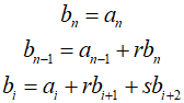
When the division is performed, a remainder $R = {b_0}$ is produced. These coefficients can have a recursive relationship.

It $t$ is indeed a root of the original polynomial, the remainder ${b_0}=0$. To compute complex roots, Bairstow's method divides the polynomial by a quadratic polynomial $B$. Applying this to the given equation yields a new polynomial.

Similar to conventional synthetic division, simple recursive relations can be used to perform division by a quadratic polynomial.
If $x-s$ is the exact divisor of the polynomial, the complex roots can be determined using the quadratic formula. Therefore, this method reduces to finding the values of $r$ and $s$ that make the remainder term zero. To eliminate the remainder, both ${b_0}$ and ${b_1}$ must be zero. Because the initial estimates of $r$ and $s$ are unlikely to make ${b_0}$ and ${b_1}$ zero, the estimates must be continuously adjusted until ${b_0}$ and ${b_1}$ are close to zero. For this, Bairstow's method approaches similarly to the Newton-Raphson method. Since ${b_0}$ and ${b_1}$ are functions of $r$ and $s$, they can be expanded using a Tayler series.

Next, use the Taylor series representing ${b_0}$ and ${b_1}$ to linearize the equations, and through this, calculate new estimates. Finally, use the Newton-Raphson iterative procedure to find new estimated that bring ${b_0}$ and ${b_1}$ closer to zero. Repeat this process to adjust the values of $r$ and $s$, continuing until ${b_0}$ and ${b_1}$ nearly converge to zero.

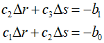
If the partial derivatives of $b$ can be determined, this results in two equations that can be solved simultaneously for the two unknowns, $\Delta r$ and $\Delta s$. Bairstow can obtain the partial derivatives of $b$ in a manner similar to how $b$ itself is derived.
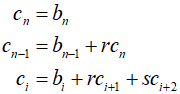
Here, $\partial {b_0}/\partial r = {c_1},\,\,\,\partial {b_0}/\partial s = \partial {b_1}/\partial r = {c_2}$, and $\partial {b_1}/\partial s = {c_3}$. Therefore, the partial derivatives are obtained through the synthetic division of $b$. These partial derivatives can then be substituted into the equations along with $b$ to solve for the values.
These equations can be solved for $\Delta r$ and $\Delta s$ to improve the initial estimates of $r$ and $s$. At each step, the approximate error for $r$ and $s$ can be estimated, and the calculations can be performed as follows.
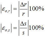
If these error estimates fall below a specified stopping criterion, the values of the roots can be determined.

When the division involves a polynomial of third degree or higher, Bairstow's method is applied to the remainder to calculate new values for $r$ and $s$. The previous values of $r$ and $s$ can be used as initial estimates for this application. If the division is of a quadratic polynomial, the remaining two roots can be directly calculated using the quadratic equation. In the case of a linear polynomial, the remaining single root can be simply calculated.
'Numerical Methods' 카테고리의 다른 글
| 138_Naive Gauss Elimination (0) | 2024.04.16 |
|---|---|
| 137_Bairstow's Method Example (0) | 2024.04.15 |
| 135_Muller's Method Example (0) | 2024.04.13 |
| 134_Muller's Method (0) | 2024.04.12 |
| 133_Newton-Raphson Method (0) | 2024.04.11 |