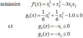
In this post, I'll solve an example using the the SQP algorithm described in the previous post.
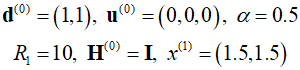
Starting point is $(1,1)$, ${R_0}=10$, $\gamma = 0.5$, and $\varepsilon = 0.001$.
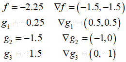
The initial iteration of the SQP algorithm is identical to the CSD algorithm. The result of the first iteration is as follows.
At ${x^2}$, the gradients for the cost function and constraints are calculated as follows.
Calculate the design change vector using the updated Hessian and step size.
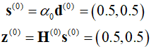
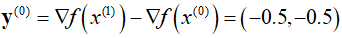
Since the Lagrange multipliers are $(0,0,0)$, the gradient of the Lagrangian is the same as the gradient of the cost function. Therefore, the vector ${{\bf{y}}^{(0)}}$ is as follows.
The scaler values required for calculation are computed as follows.
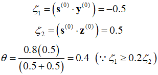
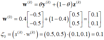
Therefore,
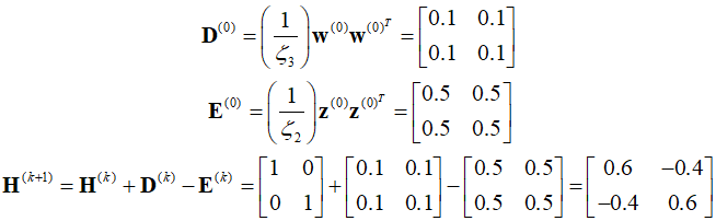
Therefore, the correction matrix and Hessian are calculated as follows.
With the updated Hessian and calculated values, the QP subproblem can be defined as follows.
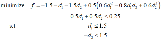
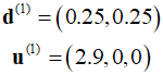
The subproblem is strictly convex, so it has a global minimum. Using the KKT conditions, the following solution can be obtained.
Subsequent calculations are performed in the same way.
'Optimization Technique' 카테고리의 다른 글
| 131_Sequential Quadratic Programming (0) | 2024.04.09 |
|---|---|
| 130_Projection Methods (0) | 2024.04.08 |
| 129_Optimality Conditions (0) | 2024.04.07 |
| 128_Step Size in the Steepest-Descent Method (0) | 2024.04.06 |
| 127_Search Direction (0) | 2024.04.05 |