Constrained optimization problems can be transformed into unconstrained problems using penalty or Lagrangian approaches. In this case, explicitly handling boundary constraints for variables in numerical optimization algorithms can be more efficient.
A constrained optimization problem can be defined as follows.
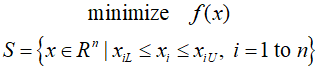
For the ${i^{th}}$ variable, ${x_{iL}}$ and ${x_{iU}}$ represent the lower and upper bounds, respectively. To observe the Karush-Kuhn-Tucker (KKT) optimality conditions for the above problem, the Lagrangian function can be defined as follows.

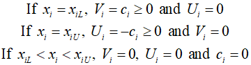
Where ${V_i}$ and ${U_i}$ are the Lagrange multipliers for the lower and upper bound constraints, respectively. The optimality conditions are as follows.

These conditions can be expressed for a stationary point as follows.
In numerical algorithms for solving the original problem, the active constraint set is not known a priori and can be determined using the following steps to decide the set of active constraints and the solution point.
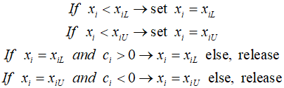
Once a variable is released, its value can move away from the boundary. Therefore, in any iteration of the numerical algorithm, the sign of the derivative of $f(x)$ with respect to a variable determines whether that variable remains at its boundary. In the next post, I"ll delve deeper into this concept through an algorithm.
'Optimization Technique' 카테고리의 다른 글
| 131_Sequential Quadratic Programming (0) | 2024.04.09 |
|---|---|
| 130_Projection Methods (0) | 2024.04.08 |
| 128_Step Size in the Steepest-Descent Method (0) | 2024.04.06 |
| 127_Search Direction (0) | 2024.04.05 |
| 126_Potential Constraint Set (0) | 2024.04.04 |