When defining the subproblem for determining the search direction in nonlinear problems, algorithms that only use linear approximations of cost and constraint functions may have the drawback of slow convergence rates. Incorporating second-order information about the problem functions into the solution process can improve this.
The Sequential Quadratic Programming (SQP) method, which I'll discuss now, uses the same approach as the previously explained unconstrained quasi-Newton methods. However, instead of using the gradient of the cost function at two points to create an approximate Hessian of the cost function, it uses the gradient of the Lagrange function at two points to update the approximate Hessian of the Lagrange function.
SQP methods can be varied in many ways, but in this post, I'll extend the constrained steepest descent algorithm to include the Hessian of the Lagrange function.
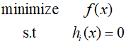
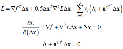
Typically, the QP subproblem, considering only design optimization problems with equality constraints, can be derived as follows.
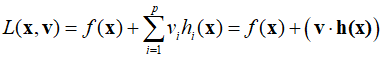
If all functions are twice continously differentiable and all constraint gradients are linearly independent, then the Lagrange function can be written as follows.
The KKT necessary conditions are as follows.
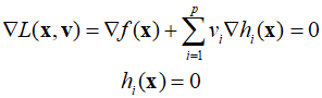
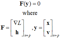
Since the design variable vector has a dimension of $n$, it represents $n$ equations. These equations, together with $p$ equality constraints, comprise $n+p$ unknowns. As these are nonlinear equations, they can be solved using the Newton-Raphson method. The above expression can be succinctly represented as follows.
Assuming ${{\bf{y}}^{(k)}}$ is known and $\Delta {{\bf{y}}^{(k)}}$ is desired, using the Taylor expansion, $\Delta {{\bf{y}}^{(k)}}$ is given as the solution to a linear system as follows.
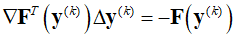
Here, $\nabla {\bf{F}}$ is the Jacobian matrix for the nonlinear equation, and substituting the definitions of ${\bf{F}}$ and ${\bf{y}}$ into the equation results in the following.
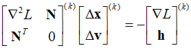
This eqaution can be transformed as follows.
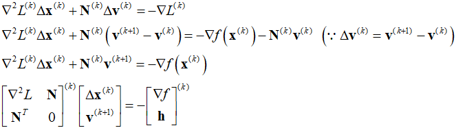
Solving the equation allows to obtain the change in design variables and the new values for the Lagrange multiplier vector. Additionally, we can see that the equation also becomes the solution to a specific QP problem defined in the $k$th iteration.
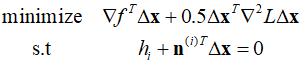
The Lagrange function and KKT necessary conditions can be written as follows.
When these equations are combined and written in matrix form, the same result is obtained.
'Optimization Technique' 카테고리의 다른 글
| 132_SQP Example (0) | 2024.04.10 |
|---|---|
| 130_Projection Methods (0) | 2024.04.08 |
| 129_Optimality Conditions (0) | 2024.04.07 |
| 128_Step Size in the Steepest-Descent Method (0) | 2024.04.06 |
| 127_Search Direction (0) | 2024.04.05 |