In the previous post, I saw the equation for projecting the design variable vector onto the constraint hyperplane. This approach is part of what's known as projection methods, like the projected conjugate gradient method, projected BFGS method, etc. The basic idea of projection methods is to fix the variables at the boundary to their boundary values in each iteration, as long as they satisfy the conditions. Subsequently, the problem is reduced to an unconstrained problem for the remaining variables. Then, methods like the conjugate gradient method or quasi-Newton methods can be used to calculate the search direction for the free variables. A line search is then performed to update the design variables. This process allows for the final active variable set to be identified quite rapidly.
To specify a numerical algorithm, it can be defined as follows.
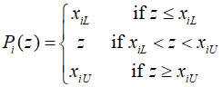
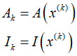
This operator ensures that all design variables are within or on their boundaries. Setting the active variable as ${A_k} = A\left( {{x^{(k)}}} \right)$, the process can be outlined as follows.
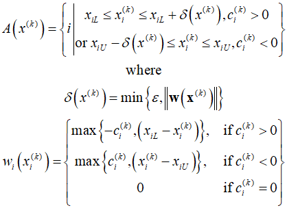
The active set ${A_k}$ includes a list of variables that are on or near the boundaries. Through the procedure outlined above, the set of active variables can be quickly identified.
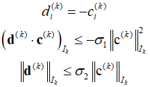
To explain the algorithm simply, consider a situation where variables are activated or deactivated according to specific constraints. First, set the iteration count $k$ to zero, calculate the gradient of the function ${{\text{c}}^{(k)}} = \nabla f\left( {{x^{(k)}}} \right)$ at the current point, and use this to define the sets of active ${A_k}$ and inactive ${I_k}$ variables.
If during this process, satisfied that a variable is within the boundary of the constraint or not exceed the boundary, the algorithm is terminated. Otherwise, the process continues.
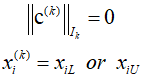
Subsequently, the steepest descent direction for the active variables is calculated. For the inactive variables, the search direction can be determined through methods such as steepest descent or conjugate gradient.
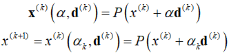
Based on this results, the design is updated using the projection operator for the step size.
Then, increment $k$ and repeat the above process. Through this method, it's possible to identify the accurate active set within a finite number of iterations and converge to a local minimum from any starting point.
ref: Schwartz, A., and E. Polak. "Family of projected descent methods for optimization problems with simple bounds." Journal of Optimization Theory and Applications 92 (1997): 1-31.
'Optimization Technique' 카테고리의 다른 글
| 132_SQP Example (0) | 2024.04.10 |
|---|---|
| 131_Sequential Quadratic Programming (0) | 2024.04.09 |
| 129_Optimality Conditions (0) | 2024.04.07 |
| 128_Step Size in the Steepest-Descent Method (0) | 2024.04.06 |
| 127_Search Direction (0) | 2024.04.05 |