In the previous post, we covered basic and popular distribution methods, and in this post, we will study one of the most important probability distributions for continuous variables, the Gaussian distribution.
The Gaussian distribution for a single real-valued variable $x$ can be defined as follows.
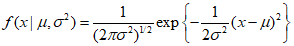
The Gaussian distribution represents the probability density for $x$ with two parameters, referred to as the mean $\mu $ and the variance ${\sigma ^2}$. Here, the square root of the variance, $\sigma$ is the standard deviation, and the reciprocal of the variance, $\beta $ represents precision.
Through the above equation, the following is satisfied.

In the Gaussian distribution, the expected values of functions of $x$ can be easily calculated, and the mean value of $x$ is as follows.
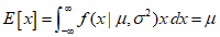
$\mu$ represents the mean value of $x$ in the distribution, hence it is referred to as the mean. The above equation is the first moment of the distribution. Similarly, calculating the second moment yields the following.
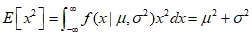
From the above two equations, the variance of $x$ is as follows.

In the case of the Gaussian distribution, the mode coincides with the mean.
When we have a dataset composed of $N$ observations with the mean and variance of the Gaussian distribution unknown, the problem of estimating the probability distribution from this dataset is known as probability density estimation.
However, the problem of estimating a probability distribution from a giben finite set of observations is not clear-cut, bacause there are an infinite number of possible probability distributions that could arise from a finite dataset.
Therefore, in such problems, we often resolve the probability distribution using a Gaussian distribution.
When the observations $x$ are independent and identically distributed, given $\mu$ and ${\sigma ^2}$, the probability of the dataset can be expressed as follows.

When viewed as a function of $\mu$ and ${\sigma ^2}$, this is known as the Gaussian likelihood function. One common method for determining the parameters within a probability distribution using an observed dataset is maximum likelihood, which involves maximizing the parameter values for the observed data. In practice, it is more common to maximize the log of the likelihood function, as maximizing the log of a function is equivalent to maximizing the function itself.
Taking the logarithm simplifies mathematical analysis and also helps improve numerical precision in computations. The log likelihood function can be expressed as follows.

Maximizing the above equation with respect to $\mu$ yields the following maximum likelihood solution.

This is the average of the observed values, and similarly, maximizing with repect to ${\sigma ^2}$ yields the maximum likelihood solution for the variance.
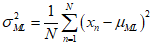
The above equation is measured as the sample variance about the sample mean. In the case of the Gaussian distribution, since the solution for $\mu$ is separate from that for ${\sigma ^2}$, the results should be used sequentially.
ref : Chris Bishop's "Deep Learning - Foundations and Concepts"
'Deep Learning' 카테고리의 다른 글
| 55_Likelihood Function (0) | 2024.01.24 |
|---|---|
| 54_Linear Regression (0) | 2024.01.23 |
| 53_Bernoulli, Binomial, and Multinomial Distribution (0) | 2024.01.22 |
| 51_Distribution (0) | 2024.01.20 |
| 50_Probability (0) | 2024.01.19 |