Before delving deeply into deep learning, I have been posting about important foundational knowledge, and today we will study linear regression models through a very simple neural network example.
Regression involves predicting one or more target variable values, $t$, when given input variables in the form of an $N$-dimensional vector. In typical supervised learning, a model is trained using a set of training data composed of ${x_n}$ training data points and corresponding target values ${t_n}$, and then used to predict the value of $t$ for new of $x$.
To acheieve this, a function with parameters that can be learned from the training data is defined.
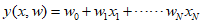
Here, $x = {({x_1} + \cdots + {x_N})^T}$, and $w$ is the linear parameter. This function can be extended as a linear combination of nonlinear functions, as follows.

Where ${{\phi _j}(x)}$ is the basis function. For convenience, we typically set ${w_0}=0$, representing the equation as follows.

Where ${\text{w}} = {({w_0}, \cdots ,{w_{M - 1}})^T}$ and $\phi = {({\phi _0}, \cdots ,{\phi _{M - 1}})^T}$. By using nonlinear basis functions, the function $y(x,w)$ can be made into a nonlinear function of the input vector $x$. However, since the function expanded as a linear combination of nonlinear functions is linear with respect to $w$, it is referred to as a linear model. Therefore, the linearity of parameters is very important in this class of models.
Before deep learning or deep neural networks became well-known, it was common in machine learning to use feature extraction, which is a fixed preprocessing form of the input variable $x$. Feature extraction involved representing through a set of basis functions and using network models to create an optimized set of these functions. However, there were limitations as problems became more complex.
In deep learning, this was addressed by learning the necessary nonlinear transformations directly from the data.

In the above formula, ${\mu _j}$ adjusts the position of the basis functions in the input space, and $s$ controls the scale. These functions are typically called Gaussian basis functions and are commonly used by multiplying them with a learnable parameter ${w_j}$.
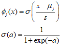
The above formula represents the form of a sigmoid basis function, where $\sigma $ is the logistic sigmoid function. Similarly, it can also be represented using the $\tanh $ function. Therefore, a general linear combination of logistic sigmoid functions can represent the same class as a general linear combination of $\tanh$ functions.
ref : Chris Bishop's "Deep Learning - Foundations and Concepts"
'Deep Learning' 카테고리의 다른 글
| 56_Sequential Learning (1) | 2024.01.25 |
|---|---|
| 55_Likelihood Function (0) | 2024.01.24 |
| 53_Bernoulli, Binomial, and Multinomial Distribution (0) | 2024.01.22 |
| 52_Gaussian Distribution (0) | 2024.01.21 |
| 51_Distribution (0) | 2024.01.20 |