I remembered that in my previous post(13_Pendulums) I said that I would explain the Finite Element Method(FEM) later.
13_Pendulums
There are a lot of interesting examples in the RADIOSS example, so I'll be working through them for a while. In this post, I'll going to perform a Pendulums example. There was also an example file in HyperMesh's installation path. However, due to the diffe
finite-elem.tistory.com
In this category, I'll talk about FEM.
I base my study on the book "A First Course in the Finite Element Method - Daryl L. Logan" and other literature
FEM is a numerical method for solving boundary value problems of differential equations.
Rather than compute the equation for the entire continuum at once, discretize it, connecting the interpolation functions of each element to approximate the overall function. Therefore, we are solving a system of approximated polynomials.
Because it is an approximate solution, it is an approach that minimizes the error from the actual solution.
Formulation of Finite Element Analysis(FEA)
Using Newton's second law, which describes states of motion on a continuum, the governing equations can be expressed as a partial differential equation in strong from.

where $\sigma $ is stress tensor, ${{\text{f}}_{\text{b}}}$ is body force.
The above expression applies to the interior points of the continuum, but in a boundary value problem where the condition must also be satisfied at the boundary.
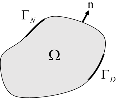
Therefore, it is necessary to consider the internal domain $\Omega $ along with the portion ${\Gamma _D}$ where Dirichlet boundary conditions are applied, and the portion ${\Gamma _N}$ where Neumann boundary conditions are imposed.
The equation considering the conditions of internal domain and boundary is as follows.

where ${\text{u}}$ is the displacement vector, ${\bar{\text u}}$ is the displacement applied to ${\Gamma _D}$, ${\text{n}}$ is the normal vector at the boundary and ${\bar{\text t}}$ is the stress vector applied to ${\Gamma _N}$.

Hooke's Law can be used to express the stress tensor in terms of the strain tensor.

where ${\text{C}}$ is the stiffness tensor, $\varepsilon $ is the strain tensor.
To apply FEM, a test function(${\text{v}}$) are used to transform into the weak form.

The above equation can be transformed as follows using the Divergence Theorem and the Fundamental Theorem of Calculus.


It the entire domain $\Omega $ is discretized into finite elements with the displacement vector in each element denoted as ${{\text{u}}_{\text{e}}}$, the linearization can be achieved using ${\text{B}}$, the partial derivative of $\varepsilon $ with respect to ${\text{u}}$

The test function is set as an interpolation function(${\text{N}}$) and substituted.

Therefore, the element stiffness matrix and the elemet load vector can be represented by the following equations.

By assembling the above equations for all elements using the following formula, the global stiffness matrix and the global load vector can be obtained.

'Finite Element Method' 카테고리의 다른 글
| 23_2D Stress and Strain (1) | 2023.12.23 |
|---|---|
| 19_Weighted residual methods (0) | 2023.12.19 |
| 18_Principle of virtual work (0) | 2023.12.18 |
| 17_Direct Methods examples (0) | 2023.12.17 |
| 16_Direct Methods (0) | 2023.12.16 |