Most numerical optimization methods calculate design changes by solving a subproblem obtained through the linear Taylor expansion of cost and constraint functions at every iteration. This idea of approximating or linearizing the subproblem is crucial in numerical optimization methods and needs to be understood.
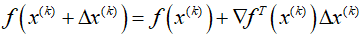
Every search method starts with an initial estimate of the design and iteratively improves it. In the $k$th iteration, if we denote the design estimate as ${x^{(k)}}$ and the change in design as $\Delta {x^{(k)}}$, a linearized subproblem can be obtained through the quadratic Tayor expansion of cost and constraint functions at the point ${x^{(k)}}$.
The linearized equality constraint is as follows.

And the linearized inequality constraint is

Where $\nabla f$, $\nabla h$, and $\nabla g$ represent the gradients of the cost function, equality constraints, and inequality constraints, repectively, and all functions and gradients are calculated at the current point ${x^{(k)}}$.
In this post, instead of a theoretical derivation, I intend to write about the notation realted to the linearized subproblem.
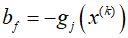
Cost function value

The $j$th equality constraint function value

The $j$th inequality constraint function value
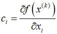
Derivative of the cost function
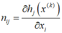
Derivative of ${h_{j}}$
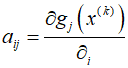
Derivative of ${g_{j}}$
Design change

Using this notation, the first equation can be defined as follows.

The linearized equality constraints
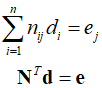
The linearized inequality constraints.

$f$ represents the linearized change of the original cost function, while ${{\bf{n}}^{(j)}}$ and ${{\bf{a}}^{(j)}}$ represent the gradients of the $j$th equality and the $j$th inequality constraint, respectively. Hence, when represented as column vectors, they are as follows.

'Optimization Technique' 카테고리의 다른 글
| 126_Potential Constraint Set (0) | 2024.04.04 |
|---|---|
| 125_Linearized Subproblem (0) | 2024.04.03 |
| 123_BFGS Method Example (0) | 2024.04.01 |
| 122_BFGS Method (0) | 2024.03.31 |
| 121_DFP Method Example (0) | 2024.03.30 |