Today, I plan to implement the same MNIST classification problem that was previously solved using a DNN in PyTorch(100_DNN Example using PyTorch), but this time using TensorFlow's Keras.
After that post, I've made some modifications to the final code(103_Code Modification) to adapt it for Keras.
First, Import the necessary libraries.
import tensorflow as tf
from tensorflow import keras
from tensorflow.keras import layers, models
from tensorflow.keras.utils import to_categorical
import matplotlib.pyplot as plt
import time
tf.random.set_seed(42)
Similar to PyTorch, in TensorFlow, I've also set the random seed to ensure that the same results are produced every time.
(x_train, y_train), (x_test, y_test) = keras.datasets.mnist.load_data()

x_train = x_train.reshape(-1, 28*28).astype('float32') / 255
x_test = x_test.reshape(-1, 28*28).astype('float32') / 255

y_train = to_categorical(y_train, 10)
y_test = to_categorical(y_test, 10)
The data to be used is loaded as follows. I used "load_data" to load the data, vectorized it, and then used "to_categorical" to convert the labels into one-hot encoding format.
The model implementataion was written in the following functional form.
def build_model(n_layer, feature, dropout):
    steps = n_layer - 1
    reduce = max(steps // feature // 64, 1)

    model = models.Sequential()
    model.add(layers.Dense(feature, activation = 'relu', input_shape=(28*28,)))
    model.add(layers.Dropout(rate=dropout))

    for i in range(n_layer - 1):
        if (i+1) % reduce == 0 and feature //2 >= 64:
            next_feature = feature // 2
        else:
            next_feature = feature
        model.add(layers.Dense(next_feature, activation = 'relu'))
        model.add(layers.Dropout(rate=dropout))
    model.add(layers.Dense(10, activation = 'softmax'))
    return model
Using Sequential in Keras allowed for a very convenient and visually clear model configuration.
I think the biggest difference from PyTorch is that in PyTorch, I have to specify both input and output dimensions for all hidden layers. However, with Keras, it was only necessary to specify the input dimension for the input layer and the output dimension for the output layer, making the process much easier then before.
Additionally, being able to specify the activation function within the Dense layer was also a significant advantage.
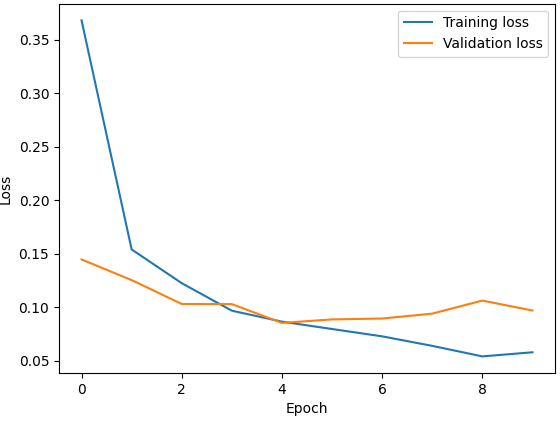
The code for model compilation and plotting the results is as follows.
model = build_model(n_layer, feature, dropout)
model.compile(optimizer='adam',
              loss='categorical_crossentropy',
              metrics=['accuracy'])
start_time = time.time()
history = model.fit(x_train, y_train, batch_size=batch_size,
                    epochs=epochs, validation_data=(x_test,y_test))
print("Total time:", time.time() - start_time)

plt.plot(history.history['loss'], label = "Training loss")
plt.plot(history.history['val_loss'], label = 'Validation loss')
plt.xlabel('Epoch')
plt.ylabel('Loss')
plt.legend()
plt.show()
In PyTorch, it was necessary to write a function for training to output the loss values separately, requiring code to be written for each step. However, in Keras, it's much simpler and easier because I can select the optimizer and loss values through "compile", and conduct training with "fit".
As a result, the entire code could be written very simple.
import tensorflow as tf
from tensorflow import keras
from tensorflow.keras import layers, models
from tensorflow.keras.utils import to_categorical
import matplotlib.pyplot as plt
import time
tf.random.set_seed(42)

def main(batch_size, n_layer, feature, epochs, dropout):
    (x_train, y_train), (x_test, y_test) = keras.datasets.mnist.load_data()

    x_train = x_train.reshape(-1, 28*28).astype('float32') / 255
    x_test = x_test.reshape(-1, 28*28).astype('float32') / 255

    y_train = to_categorical(y_train, 10)
    y_test = to_categorical(y_test, 10)

    model = build_model(n_layer, feature, dropout)
    model.compile(optimizer='adam',
                  loss='categorical_crossentropy',
                  metrics=['accuracy'])
    start_time = time.time()
    history = model.fit(x_train, y_train, batch_size=batch_size,
                        epochs=epochs, validation_data=(x_test,y_test))
    print("Total time:", time.time() - start_time)

    plt.plot(history.history['loss'], label = "Training loss")
    plt.plot(history.history['val_loss'], label = 'Validation loss')
    plt.xlabel('Epoch')
    plt.ylabel('Loss')
    plt.legend()
    plt.show()

def build_model(n_layer, feature, dropout):
    steps = n_layer - 1
    reduce = max(steps // feature // 64, 1)

    model = models.Sequential()
    model.add(layers.Dense(feature, activation = 'relu', input_shape=(28*28,)))
    model.add(layers.Dropout(rate=dropout))

    for i in range(n_layer - 1):
        if (i+1) % reduce == 0 and feature //2 >= 64:
            next_feature = feature // 2
        else:
            next_feature = feature
        model.add(layers.Dense(next_feature, activation = 'relu'))
        model.add(layers.Dropout(rate=dropout))
    model.add(layers.Dense(10, activation = 'softmax'))
    return model

if __name__ == "__main__":
    batch_size = 128
    n_layer = 5
    feature = 1024
    epochs = 10
    dropout = 0.3
    main(batch_size, n_layer, feature, epochs, dropout)
The final results are as follows.

Training Loss : 0.0581
Validation Loss : 0.0880
Time : 42.21s
I having primarily used PyTorch for constructing neural networks, I find that using Keras makes the process fell much easier.
'Deep Learning' 카테고리의 다른 글
| 164_K-fold Cross Validation (0) | 2024.05.13 |
|---|---|
| 163_Basic Graph Properties (0) | 2024.05.12 |
| 103_Code Modification (0) | 2024.03.12 |
| 102_Dropout Layers (0) | 2024.03.11 |
| 101_Overfitting (0) | 2024.03.10 |