In a previous post, we implemented an ANN (Artificial Neural Network) with a simple single hidden layer. In this post, we aim to solve a classification problem using a DNN (Deep Neural Network) with more than two hidden layers, continuing with the MNIST dataset used before.
First, let's import the necessary libraries.
import torch
import torchvision
import torchvision.transforms as transforms
from torch.utils.data import DataLoader, random_split
import torch.optim as optim
from tqdm import tqdm
import matplotlib.pyplot as plt
import time

torch.manual_seed(42)
Actually, other than the model, all other aspects are identical to the previous ANN code.
train_set = torchvision.datasets.MNIST(root='./data', train=True, download = True,
                                       transform=transforms.Compose([transforms.ToTensor()]))

training_size = int(0.8*len(train_set))
validation_size = len(train_set)-training_size
training_dataset, validation_dataset = random_split(train_set, [training_size, validation_size])

training_loader = DataLoader(training_dataset, batch_size= 64, shuffle = True)
validation_loader = DataLoader(validation_dataset, batch_size=64)
Load the data and split it into training data and validation data. The batch size is 64.
Then, create the DNN model.
class DNN(torch.nn.Module):
    def __init__(self):
        super(DNN, self).__init__()
        self.input = torch.nn.Linear(28*28, 512)
        self.hidden1 = torch.nn.Linear(512, 256)
        self.hidden2 = torch.nn.Linear(256, 128)
        self.hidden3 = torch.nn.Linear(128, 64)
        self.output = torch.nn.Linear(64, 10)

    def forward(self, x):
        x = x.view(-1, 28*28)
        x = torch.relu(self.input(x))
        x = torch.relu(self.hidden1(x))
        x = torch.relu(self.hidden2(x))
        x = torch.relu(self.hidden3(x))
        x = self.output(x)
        return x
In fact, the part about the model being different from the ANN is only in terms of the number of hidden layers, otherwise, it's the same ;). In this model, three hidden layers are stacked, each consisting of 512, 256, and 128 nodes, respectively.
def train(model, training_loader, validation_loader, epochs = 10):
    training_losses = []
    validation_losses = []

    criterion = torch.nn.CrossEntropyLoss()
    optimizer = optim.Adam(model.parameters())

    for epoch in range(epochs):
        model.train()
        running_loss = 0.0
        for inputs, labels in tqdm(training_loader, desc=f"Epoch {epoch+1}/{epochs}"):
            optimizer.zero_grad()
            outputs = model(inputs)
            loss = criterion(outputs, labels)
            loss.backward()
            optimizer.step()
            running_loss += loss.item()
        training_losses.append(running_loss / len(training_loader))

        model.eval()
        validation_loss = 0.0
        with torch.no_grad():
            for inputs, labels in validation_loader:
                outputs = model(inputs)
                loss = criterion(outputs, labels)
                validation_loss += loss.item()
        validation_losses.append(validation_loss / len(validation_loader))

        print(f'Epoch {epoch+1}, Training Loss: {training_losses[-1]:.4f}, Validation Loss: {validation_losses[-1]:.4f}')

    return training_losses, validation_losses
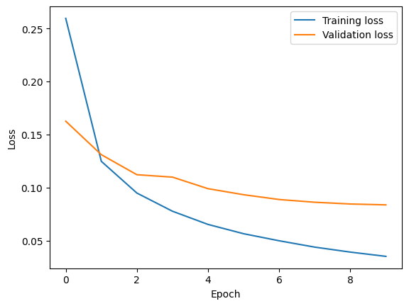
As with the previous code, training is conducted for 10 epochs, and progress is monitored using tqdm. At the end of each epoch, the training loss and validation loss are printed.
s = time.time()
model = DNN()
training_losses, validation_losses = train(model, training_loader, validation_loader)
print("total time : ",time.time()-s)
plt.plot(training_losses, label='Training loss')
plt.plot(validation_losses, label='Validation loss')
plt.xlabel('Epoch')
plt.ylabel('Loss')
plt.legend()
plt.show()
Compare the results with the ANN.
ANN
Training Loss : 0.0351
Validation Loss : 0.0836
Time : 70.6s

DNN
Training Loss : 0.0203
Validation Loss : 0.1044
Time : 82.2s

Compared to the ANN, the DNN showed a reduction in Training loss, but as training progressed, it demonstrated a decreased ability to predict on the Validation Data accurately, indicating that overfitting occurred.
In the next post, we plan to address overfitting and modify the code to make it more readable and efficient.
As an aside, today marks the 100th day since I opened the blog and began writing posts daily. I'm proud of myself for consistently realizing a plan that started with nothing, and I'm happy to see that I'm doing well.
Congratulation on the 100th post!
'Deep Learning' 카테고리의 다른 글
| 102_Dropout Layers (0) | 2024.03.11 |
|---|---|
| 101_Overfitting (0) | 2024.03.10 |
| 99_Simple CNN Example Using PyTorch (0) | 2024.03.08 |
| 98_Simple ANN Example Using PyTorch(2) (0) | 2024.03.07 |
| 97_Simple ANN Example Using PyTorch (0) | 2024.03.06 |