In this post, we will conduct a simple CNN (Convolutional Neural Network) example in a PyTorch environment using the MNIST dataset. In a previous post (97_Simple DNN Example Using PyTorch), we addressed the same classification problem using a DNN (Deep Neural Network), and with slight modifications, it can be adapted to a CNN. For an explanation of CNN, please refer to another post (69_Convolutional Filter).
MNIST is a large-scale dataset composed of handwritten digits, widely used in the fields of machine learning and computer vision for training and testing image processing algorithms. MNIST consists of digits from 0 to 9.
And MNIST is widely used as a standard benchmark for comparing and evaluating the performance of algorithms, using a deep learning framework like PyTorch allows for the easy loading and use of the MNIST dataset.
Fisrt, import the necessary libraries.
import torch
import torchvision
import torchvision.transforms as transforms
from torch.utils.data import DataLoader, random_split
import torch.nn as nn
import torch.optim as optim
from tqdm import tqdm
import matplotlib.pyplot as plt
import time

torch.manual_seed(42)
Similar to the previous post, but with a difference the 'time' module was imported to assess the required time, and to ensure consistent results, the manual seed for 'torch' was set.
train_set = torchvision.datasets.MNIST(root='./data', train=True, download = True,
                                       transform=transforms.Compose([transforms.ToTensor()]))

train_size = int(0.8 * len(train_set))
validation_size = len(train_set) - train_size
train_dataset, validation_dataset = random_split(train_set, [train_size, validation_size])

train_loader = DataLoader(train_dataset, batch_size=64, shuffle=True)
validation_loader = DataLoader(validation_dataset, batch_size=64)
Using 'torchvision.datasets', you can fetch and save the MNIST dataset. With 'transforms.Compose', it's possible to convert images to PyTorch tensor types, and the pixel values are automatically scaled to a range of 0 to 1. The ratio for training and validation has been set to 8:2, and the batch size is configured to 64.
Now, define the model.
class CNN(nn.Module):
    def __init__(self):
        super(CNN, self).__init__()
        self.conv1 = nn.Conv2d(1, 32, kernel_size=5, stride=1, padding=2)
        self.pool = nn.MaxPool2d(kernel_size=2, stride=2, padding=0)
        self.conv2 = nn.Conv2d(32, 64, kernel_size=5, stride=1, padding=2)
        self.fc1 = nn.Linear(64 * 7 * 7, 1000)
        self.fc2 = nn.Linear(1000, 10)

    def forward(self, x):
        x = self.pool(torch.relu(self.conv1(x)))
        x = self.pool(torch.relu(self.conv2(x)))
        x = x.view(-1, 64 * 7 * 7)
        x = torch.relu(self.fc1(x))
        x = self.fc2(x)
        return x
The first convolutional layer is set as 'conv1'. The input channel is 1, and the output channel is 32. The kernel size is 5*5, where the kernel represents the size of the filter. The stride, which indicates the number of pixels the filter moves across the input image in one step, is set to 1. Padding, which adds extra pixels to the edges of the input image to prevent the output feature map from becoming too small, is set to 2.
The pooling layer uses a kernel size of 2*2 with a stride of 2. It employs Max pooling, which selects the maximum value from the feature map to reduce dimensions.
The second convolutional layer is 'conv2', with the input channel being 32, matching the output channel of the previous convolutional layer. The output channel is 64, and the kernel size, stride, and padding are the same as in 'conv1'.
Afterwards, the first fully connected layer is set as 'fc1', with the number of neurons in the input set to 64*7*7. This corresponds to the size of the feature map after the second pooling, indicating there are 64 feature maps of size 7*7. The number of output neurons is set to 1000.
The second fully connected layer is set as 'fc2', with the input neuron count being the output neuron count of 'fc1', which is 1000, and the output neuron count is 10.
Lastly, the activation function used is ReLU.
The neural network training is as follows.
def train(model, train_loader, validation_loader, epochs=10):
    train_losses = []
    validation_losses = []

    criterion = nn.CrossEntropyLoss()
    optimizer = optim.SGD(model.parameters(), lr=0.01, momentum=0.9)
    for epoch in range(epochs):
        model.train()
        running_loss = 0.0
        for inputs, labels in tqdm(train_loader, desc=f"Epoch {epoch+1}/{epochs}"):
            optimizer.zero_grad()
            outputs = model(inputs)
            loss = criterion(outputs, labels)
            loss.backward()
            optimizer.step()
            running_loss += loss.item()
        train_losses.append(running_loss / len(train_loader))

        model.eval()
        validation_loss = 0.0
        with torch.no_grad():
            for inputs, labels in validation_loader:
                outputs = model(inputs)
                loss = criterion(outputs, labels)
                validation_loss += loss.item()
        validation_losses.append(validation_loss / len(validation_loader))

        print(f'Epoch {epoch+1}, Train Loss: {train_losses[-1]:.4f}, Validation Loss: {validation_losses[-1]:.4f}')
    return train_losses, validation_losses
For the loss function, CrossEntropyLoss, which is widely used in classification tasks, was utilized, and the optimizer for updating the model's parameters was SGD to minimize the model's loss.
Training proceeded for 10 epochs, and 'tqdm' was used to monitor progress within each epoch. After each epoch, the Training loss and Validation loss were printed and saved. Once all training was completed, the loss values for each were returned.
model = CNN()
train_losses, validation_losses = train(model, train_loader, validation_loader)
plt.plot(train_losses, label='Training loss')
plt.plot(validation_losses, label='Validation loss')
plt.xlabel('Epoch')
plt.ylabel('Loss')
plt.legend()
plt.show()
By executing the above code to train the model, the results are as follows.

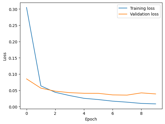
Ultimately, the Training Loss was 0.0083and the Validation Loss was 0.0390, which are significantly lower loss values compared to those obtained with the DNN.
'Deep Learning' 카테고리의 다른 글
| 101_Overfitting (0) | 2024.03.10 |
|---|---|
| 100_DNN Example using PyTorch (0) | 2024.03.09 |
| 98_Simple ANN Example Using PyTorch(2) (0) | 2024.03.07 |
| 97_Simple ANN Example Using PyTorch (0) | 2024.03.06 |
| 74_Diffusion Model(2) (0) | 2024.02.12 |