Today, I plan to solve an example using the DFP method as explained in the last post(120_Inverse Hessian Updating).

Set the initial starting point ${x^{(0)}}$ to (1,2), ${{\text{A}}^{(0)}}$ to the identity matrix, $k=0$ for the first iteration, and the stopping criterion $\varepsilon $ to 0.001. The gradient vector at the starting point can be calculated as follows.

Calculate the norm and criterion check.

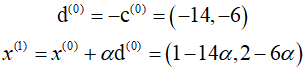
Since the norm values is greater than $\varepsilon $, change the direction of the design change and update the design variables.
Substitute the updated design variables into the Cost function and recalculate.

Insert the calculated step size to finally update the design variables.

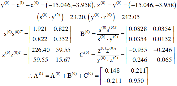
Calculate the correction matrices ${{\text{B}}^{(0)}}$ and ${{\text{C}}^{(0)}}$ using the quasi-Newton condition.
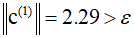
For the start of the second iteration, recalculate the norm of the gradient vector to check the criterion again.
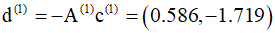
Calculate the search direction.
Calculate the step size and use the calculated value along with the search direction value to update $x$.

Based on the calculated values, compute the correction matrices.

Although this process must be repreated until convergence criteria are met, through such a procedure, we can see that a ${\text{A}}$ matrix closely approximates the inverse of the Hessian of the cost function.
'Optimization Technique' 카테고리의 다른 글
| 123_BFGS Method Example (0) | 2024.04.01 |
|---|---|
| 122_BFGS Method (0) | 2024.03.31 |
| 120_Inverse Hessian Updating (0) | 2024.03.29 |
| 119_Modified Newton Method (0) | 2024.03.28 |
| 118_Conjugate Gradient Algorithm (0) | 2024.03.27 |